

Most people’s first molecular dynamics run fails for a reason that has nothing to do with physics: a missing mass line, a units mismatch, or a timestep large enough to send atoms through each other.
So this is a tutorial with a deliberately boring goal. You will melt a block of argon, watch the temperature and energy behave sensibly, and understand what every single line of the input script is doing. Twenty minutes, no prior MD experience, and a result you can check against a known answer.
In this post:
- Installing LAMMPS without compiling anything
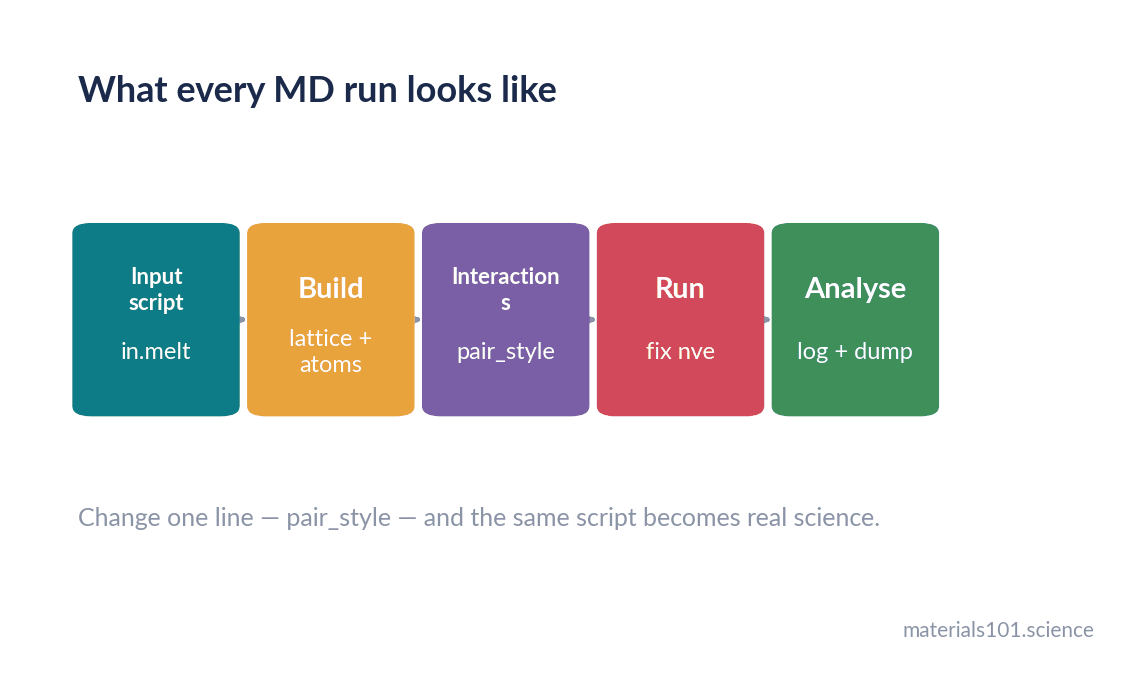
- The input script, line by line
- Running it and reading the log
- Plotting the two curves that tell you whether it worked
- The five failures that catch everyone
Install it
The simplest route on any operating system is conda:
conda create -n md -c conda-forge lammps
conda activate md
lmp -help | head -5
On Ubuntu, sudo apt install lammps also works and is fine for learning. On Windows, either use the conda route inside WSL, or download the prebuilt installer from the LAMMPS site. You do not need to compile LAMMPS to follow this post, and you do not need a GPU.
The input script, line by line
Save this as in.melt. It is the classic Lennard-Jones melt example that ships with LAMMPS, and it runs in a couple of seconds.
# 1. units and atom style
units           lj
atom_style      atomic

# 2. geometry
lattice         fcc 0.8442
region          box block 0 10 0 10 0 10
create_box      1 box
create_atoms    1 box
mass            1 1.0

# 3. interactions
pair_style      lj/cut 2.5
pair_coeff      1 1 1.0 1.0 2.5

# 4. initial state
velocity        all create 3.0 87287 loop geom

# 5. neighbour bookkeeping
neighbor        0.3 bin
neigh_modify    every 20 delay 0 check no

# 6. what is held fixed
fix             1 all nve

# 7. what gets recorded
thermo          50
thermo_style    custom step temp epair etotal press
dump            1 all atom 100 dump.melt

# 8. go
run             1000
Now the same script as decisions rather than syntax.
units lj — reduced units. Lengths are in units of σ, energies in ε, temperature in ε/k_B. Nothing is in kelvin or ångström. This is why the temperature reads 3.0 rather than 300. For a real material you would write units metal and get eV, ångström, picoseconds.
atom_style atomic — each atom is a point with a mass and a position. No charges, no bonds. Charged systems need charge, molecules need full.
lattice fcc 0.8442 — sets up an FCC lattice at a reduced density of 0.8442, which is the standard LJ liquid-triple-point density. region and create_box then define a 10 × 10 × 10 lattice-unit cube with periodic boundaries by default, and create_atoms fills it. That gives 4000 atoms, because FCC has four atoms per cubic cell.
mass 1 1.0 — the line everyone forgets. LAMMPS will not run without a mass for every atom type, and the error message does not make the reason obvious.
pair_style lj/cut 2.5 with pair_coeff 1 1 1.0 1.0 2.5 — Lennard-Jones with ε = 1.0, σ = 1.0, truncated at 2.5σ. Truncation is an approximation: beyond 2.5σ the attraction is set to zero rather than tapered, which shifts the pressure slightly. It is the conventional choice and it is what published LJ results use, so keep it if you want to compare against them.
velocity all create 3.0 87287 — draw velocities from a Maxwell-Boltzmann distribution at T = 3.0, using 87287 as the random seed. Change the seed and you get a different trajectory from the same starting structure, which is exactly how you generate independent replicas.
neighbor and neigh_modify — bookkeeping. LAMMPS keeps a list of which atoms are close enough to interact, and rebuilds it periodically. This is the single biggest reason MD scales linearly rather than as N².
fix 1 all nve — integrate Newton’s equations with constant number, volume and energy. No thermostat. Energy should be conserved; temperature will drift to whatever the system settles at. Swap in fix 1 all nvt temp 1.0 1.0 0.1 for constant temperature.
thermo 50 and thermo_style — print these quantities every 50 steps. dump writes atom positions every 100 steps so you can visualise the trajectory.
Run it
lmp -in in.melt
You will see a table like this:
Step Temp E_pair TotEng Press
0    3    -6.7733681 -2.2744931 -3.7033504
50   1.6758903 -4.7955425 -2.2823945 5.670064
100  1.6452239 -4.7492704 -2.2820623 5.8691042
...
Three things to check, in this order.
Temperature drops from 3.0 to about 1.65 and stays there. That is not a bug. You created velocities for T = 3.0 on a perfect lattice, so the system had no potential energy of disorder; as the lattice melts, kinetic energy converts to potential energy and the temperature halves. Equipartition doing its job.
Total energy stays essentially constant. In NVE it must. If TotEng drifts steadily, your timestep is too large or your neighbour settings are too loose.
Pressure is positive and roughly steady. At this density and temperature the LJ fluid is under compression.
Plot the two curves that matter
The figures below come from an independent 500-atom Lennard-Jones run written in about forty lines of NumPy, using the same potential, cutoff and integrator — it runs inside the script that draws them, so you can reproduce and modify it without LAMMPS installed at all.
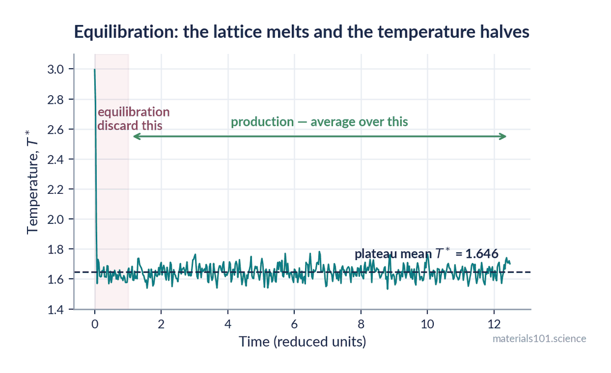
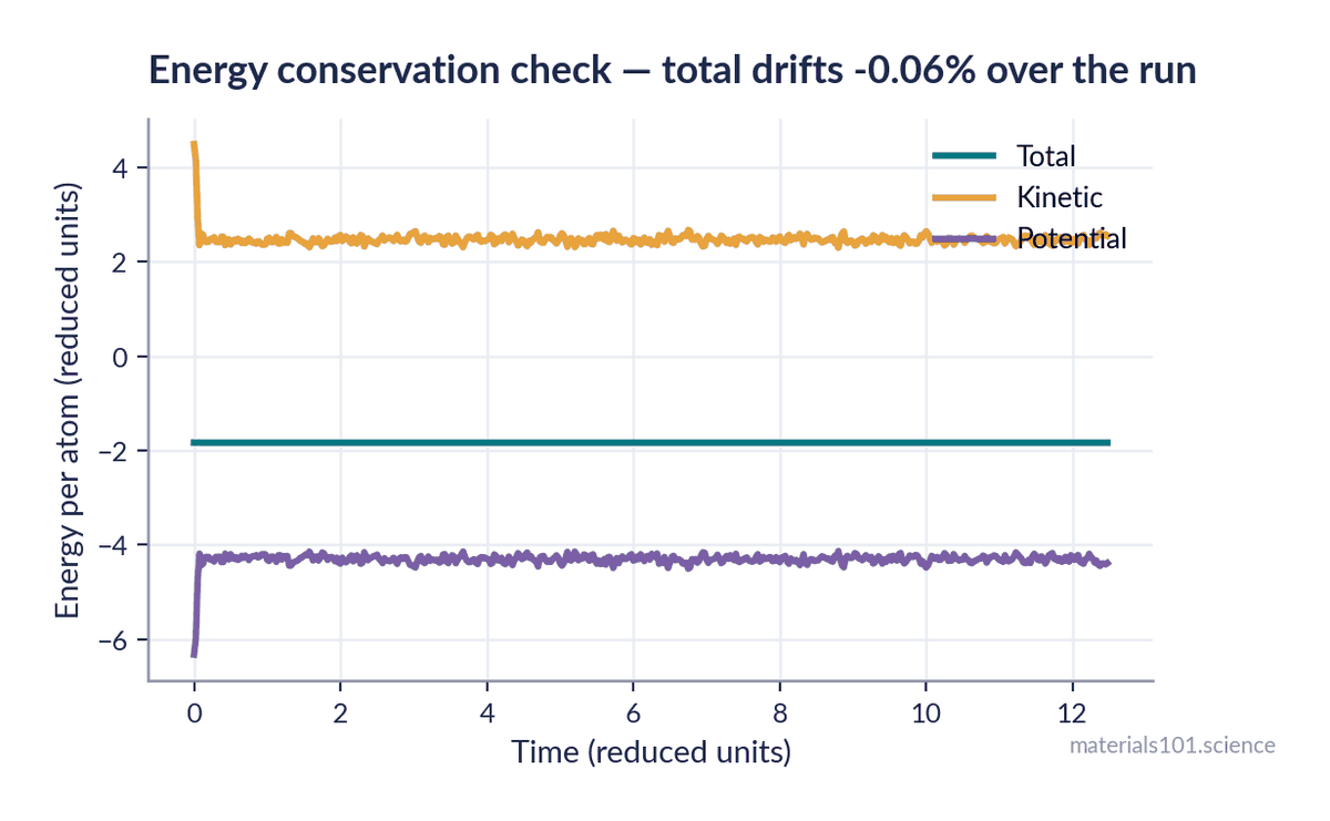
Worth noting what that independent run produces: a temperature plateau of 1.646 and a total-energy drift of −0.06% over 2,500 steps. The plateau agrees with the LAMMPS example’s own documented behaviour, from a completely separate implementation — which is the cheapest validation exercise in computational science and one worth repeating whenever you adopt a new code.
If your total energy drifts upward like a ramp, the timestep is too big. Halve it and the drift should fall by roughly a factor of four, since velocity Verlet’s energy error scales as the square of the timestep.
The five failures that catch everyone
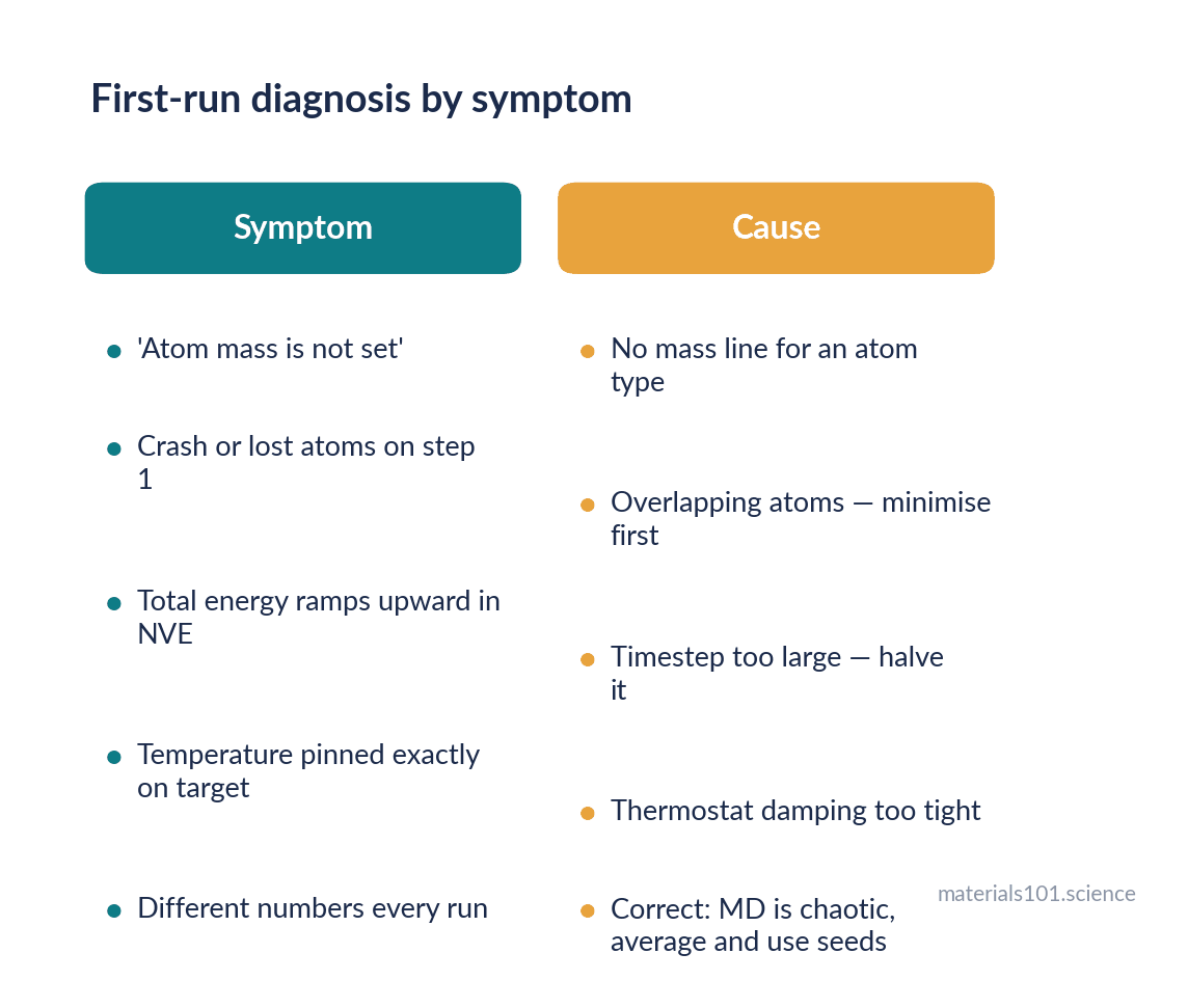
1. “Atom mass is not set” — add a mass line for every atom type. LAMMPS will not guess.
2. “Lost atoms” or a crash on step 1 — your atoms overlap, so the LJ repulsion is astronomically large and they get launched out of the box. Either your lattice spacing is too small, or you built the structure badly. Run an energy minimisation first: minimize 1.0e-4 1.0e-6 100 1000.
3. Energy climbing steadily in NVE — timestep too large. In LJ units, 0.005 is safe and 0.01 is pushing it. In metal units, 1 fs is standard, and 2 fs is the most you should attempt without constraints.
4. Temperature pinned at exactly your target, and nothing interesting happens — you are running NVT with a very tight damping constant. The thermostat is overwhelming the dynamics. Loosen the damping, or use NVE once equilibrated.
5. Results that change every run — that is correct and expected. MD is chaotic: different seeds diverge. Any quantity you report needs averaging over an equilibrated window, and ideally over several independent seeds with an error bar.
Going deeper
Two habits worth forming immediately. First, always discard the equilibration period before averaging anything — the plateau in the temperature figure shows you where it ends, and averaging across the transient will quietly bias every number you report. Second, block-average: split the equilibrated run into five or ten blocks, average each, and take the standard error across blocks. Consecutive MD frames are correlated, so the naive standard error over all frames underestimates the true uncertainty, sometimes by an order of magnitude.
In practice
The LJ melt is a test that your installation works, not science. The step up to a real material means replacing pair_style lj/cut with a potential fitted to something: an EAM file for a metal, a Tersoff or MEAM for a covalent solid, or a machine-learned potential for near-DFT accuracy. That one line change is the entire difference, and it is why the input-script structure is worth learning properly.
Common misconceptions
- “Reduced units are just a convenience.” They are dimensionless: one LJ simulation stands for every substance that obeys the LJ potential, once you know ε and σ. That is why LJ results are quoted in reduced units in the literature.
- “Longer runs are always better.” Beyond a point you are adding correlated samples, not information. Independent seeds buy you more than a longer single trajectory.
- “NVE means nothing is controlled.” Number, volume and total energy are all fixed. It is the most physically honest ensemble and the right one for checking whether your integration is sound.
Key takeaways
- An MD input script is five decisions: which atoms, where they start, how they interact, what is held fixed, and what you record.
units ljmeans every number is dimensionless — temperature 3.0 is not 3 kelvin.- In NVE, constant total energy is your correctness check; a steady drift means the timestep is too large.
- Temperature falling after startup is physics, not a bug: the lattice is melting.
- Discard the equilibration transient and block-average before reporting any number.
Frequently asked questions
How do I start learning LAMMPS?
Install it with conda, run the Lennard-Jones melt example, and read the log until you can explain every column. Then change one thing at a time — the ensemble, the timestep, the potential — and watch what happens. The LAMMPS documentation is unusually good and every command page has examples.
What timestep should I use in LAMMPS?
About 0.005 in Lennard-Jones reduced units, and 1 fs for metals in units metal. The test is whether total energy is conserved in NVE; if it drifts, halve the timestep.
Why does my temperature drop at the start of the run?
Because you assigned velocities to a perfectly ordered lattice. As the structure disorders, kinetic energy converts into potential energy and the temperature falls to roughly half its starting value. Assign twice your target temperature, or equilibrate with a thermostat.
What is the difference between NVE and NVT?
NVE conserves total energy with no thermostat, so temperature fluctuates freely. NVT holds temperature at a set value by coupling to a thermostat, which means energy is no longer conserved. Equilibrate in NVT, then measure in NVE if the property is energy-sensitive.
Do I need a GPU for molecular dynamics?
Not for learning. The example here runs in seconds on a laptop. GPUs matter when you reach millions of atoms or nanosecond-scale trajectories with an expensive potential.
Next read
- What is a machine-learned interatomic potential? — the one line that turns this tutorial into real science
- Density functional theory, explained without the math — where a potential’s training data comes from
References
The input script is the Lennard-Jones melt example distributed with LAMMPS. The
figures come from an independent NumPy implementation of the same system, run by
this post’s figure script, so both are reproducible.
- A. P. Thompson, H. M. Aktulga, R. Berger, D. S. Bolintineanu, W. M. Brown, P. S. Crozier, P. J. in ‘t Veld, A. Kohlmeyer, S. G. Moore, T. D. Nguyen, R. Shan, M. J. Stevens, J. Tranchida, C. Trott and S. J. Plimpton, LAMMPS — a flexible simulation tool for particle-based materials modeling at the atomic, meso, and continuum scales, Computer Physics Communications 271, 108171 (2022). doi:10.1016/j.cpc.2021.108171
- S. Plimpton, Fast Parallel Algorithms for Short-Range Molecular Dynamics, Journal of Computational Physics 117, 1–19 (1995). doi:10.1006/jcph.1995.1039 — the neighbour-list and spatial-decomposition methods that make this scale.
- M. P. Allen and D. J. Tildesley, Computer Simulation of Liquids, 2nd ed., Oxford University Press, 2017 — velocity Verlet, equipartition, block averaging and error estimation.
Written by Dinesh Varma, PhD scholar in computational materials science.
Spotted an error? Tell me — corrections are credited.