Write down the Schrödinger equation for a single water molecule and you have a function of 30 coordinates. Ten electrons, three spatial dimensions each. Store it on a grid with ten points per dimension and you need 1030 numbers. There is not enough matter in the solar system to build that hard drive.
Yet a laptop can predict water’s bond angle to within a degree. Density functional theory is how.
By the end of this post you will be able to explain what DFT actually computes, why it is fast enough to be useful, and which of its answers you should treat with suspicion.
In this post:
- The trick: density instead of wavefunction
- What the computer actually does, step by step
- The one approximation, and the ladder of choices
- What DFT is good at, and what it gets wrong
- The settings that decide whether your answer means anything
The trick: density instead of wavefunction
The many-electron wavefunction is a function of every electron’s position at once. Its size explodes with electron count, which is why the direct approach dies at about two atoms.
The electron density is different. It is just a number at each point in space: how much electron is here. One function, three coordinates, no matter how many electrons the system has. A copper atom and a protein both have a density you can plot on a page.
In 1964, Hohenberg and Kohn proved something that sounds too good to be true [1]. The ground-state density contains, in principle, everything about the system. Two theorems: the density uniquely determines the external potential, so it determines everything else; and the true density is the one that minimises the energy.
That is the whole conceptual foundation. Stop tracking every electron. Track how much electron sits where.
There was a catch, and it is still the catch. The theorems say the energy is a functional of the density. They do not say what that functional is.
What the computer actually does
Kohn and Sham made the idea practical in 1965 with a piece of controlled cheating [2]. Replace the real, interacting electrons with a fictitious system of non-interacting electrons that has exactly the same density. Non-interacting electrons are easy: you can write one equation per electron and solve them.
Everything the cheat leaves out — exchange, correlation, and the difference in kinetic energy between the real and fictitious systems — gets swept into a single term called the exchange-correlation functional. Get that term right and DFT would be exact. Nobody knows it exactly, so we approximate it, and every DFT calculation you will ever run is only as good as that approximation.
The calculation itself is a loop, because the equations depend on their own answer. The potential each electron feels depends on the density, and the density comes from solving for the electrons in that potential.
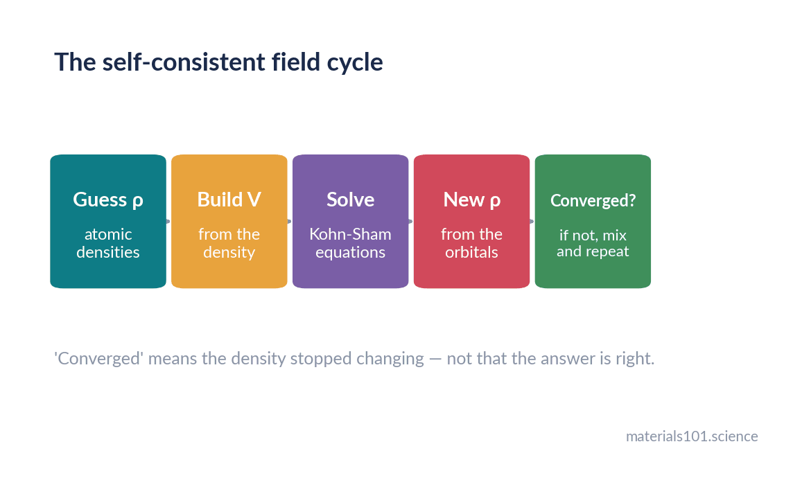
- Guess a starting density, usually by overlapping isolated-atom densities.
- Build the potential each electron sees from that density.
- Solve the Kohn-Sham equations for the orbitals in that potential.
- Rebuild the density from the occupied orbitals.
- Compare. If the new density differs from the old one, mix them and go back to step 2.
When the density stops changing, the loop has converged and you can read off the total energy, the forces on every atom, the band structure and the charge distribution. Move the atoms along those forces and repeat, and you are relaxing a structure.
Going deeper
Two practical points. First, “self-consistent” says nothing about being right — a beautifully converged SCF cycle with a bad functional gives you a precise wrong answer. Second, DFT as normally practised is a ground-state, zero-temperature theory. Finite temperature enters through phonons, thermal expansion or molecular dynamics on top of it, not through the SCF cycle itself, and excited states need something else entirely, such as time-dependent DFT or GW.
The one approximation, and how to choose it
Approximate functionals are usually described as rungs on a ladder — each rung uses more information about the density and costs more.
| Rung | Functional | Uses | Typical use |
|---|---|---|---|
| 1 | LDA | density only | fast, over-binds, historical baseline |
| 2 | GGA (PBE [3], PBEsol) | density + its gradient | the workhorse for solids |
| 3 | meta-GGA (SCAN [4], r²SCAN) | + kinetic energy density | better geometries and energetics, modest extra cost |
| 4 | hybrid (HSE06 [5], PBE0) | + exact exchange | band gaps, molecules; 10–100× the cost |
| 5 | RPA and beyond | unoccupied states | benchmark quality, expensive |
PBE is the default in most materials work for a reason: it is cheap, it is well understood, and its errors are known and fairly systematic. Lattice constants come out roughly 1% too large, cohesive energies are somewhat too small, and band gaps are underestimated by around half. That last one is not a bug you can tune away — it is a known property of the approximation, and it is why HSE06 exists.
What DFT is good at, and what it gets wrong
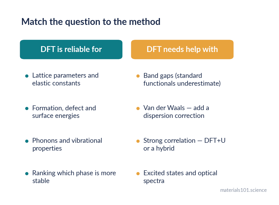
DFT is genuinely reliable for ground-state structure and energetics: lattice parameters, elastic constants, formation energies, defect energies, surface energies, phonon spectra, reaction barriers with a decent functional. For ranking candidate structures — is this phase more stable than that one — it is excellent, because systematic errors partly cancel between similar systems.
It is unreliable, or needs care, for band gaps with standard functionals, van der Waals interactions unless you add a dispersion correction such as Grimme’s D3 [6], strongly correlated systems including many transition-metal oxides where you may need DFT+U or a hybrid, and anything involving excited states or optical spectra.
In practice
If your reviewer or your supervisor asks a hard question about a DFT result, it is almost always one of four: which functional, what cutoff and k-point mesh, what pseudopotentials, and how the structure was relaxed. Report all four. A DFT number without its settings is not reproducible, and the settings are where most of the disagreement between papers actually lives.
The settings that decide whether your answer means anything
Two parameters control the numerical quality of nearly every plane-wave calculation, and neither has a universally right value.
The plane-wave cutoff energy sets how finely the wavefunctions are described. Too low and your energies are wrong; too high and you are burning CPU time for no benefit. The k-point mesh samples the Brillouin zone. Metals need much denser meshes than insulators because their Fermi surfaces need resolving.
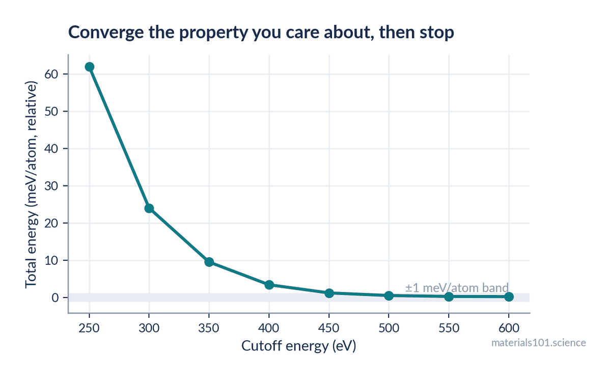
The rule is simple and often ignored: converge the property you care about, not the total energy. Total energies converge slowly; energy differences between similar structures converge much faster, and forces and stresses converge more slowly than energies. Pick a tolerance — 1 meV/atom is a common choice — and stick to the same settings across every calculation you intend to compare.
Common misconceptions
- “DFT is exact.” The theory is exact in principle; every real calculation uses an approximate exchange-correlation functional. That approximation is the dominant error, and it is a choice you make.
- “A converged calculation is a correct calculation.” Convergence means the numbers stopped changing. It says nothing about whether the functional, the pseudopotential or the starting structure was appropriate.
- “DFT band gaps are just less accurate.” Standard DFT band gaps are underestimated for a structural reason connected to the derivative discontinuity of the functional, not because of insufficient numerical effort. Throwing more cutoff at it does not help.
Key takeaways
- DFT replaces the many-electron wavefunction with the electron density, turning an impossible problem into a solvable one.
- The Kohn-Sham approach solves non-interacting equations self-consistently and hides the hard physics in the exchange-correlation functional.
- Functional choice is the dominant approximation: PBE for general solid-state work, meta-GGA for better geometries, hybrids when band gaps matter.
- DFT is strongest for ground-state structure and energetics, weakest for band gaps, dispersion and strong correlation.
- Cutoff, k-points, pseudopotentials and relaxation criteria must be converged and reported — they are where reproducibility is won or lost.
Frequently asked questions
What is density functional theory in simple terms?
DFT is a method for predicting the properties of atoms, molecules and solids by working with the electron density — how much electron sits at each point in space — instead of the full many-electron wavefunction. That swap makes quantum-mechanical accuracy affordable for hundreds of atoms.
Why is DFT called a first-principles method?
Because it needs only the atomic numbers and positions as input. No experimental data is fitted, which is why it can predict properties of materials that have never been made.
How many atoms can DFT handle?
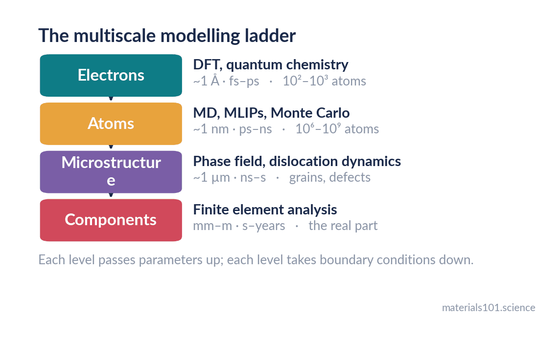
Routinely a few hundred with plane-wave codes on a normal cluster; the cost grows roughly as the cube of the number of electrons, so a thousand atoms is a serious undertaking. This is exactly the wall that machine-learned interatomic potentials were built to get past.
Which exchange-correlation functional should I use?
PBE for general solid-state work, r²SCAN when you want better geometries and formation energies at modest extra cost, and a hybrid such as HSE06 when band gaps or molecular energetics matter. Always state which one you used.
Is DFT accurate enough for real engineering?
For ranking phases, computing elastic constants, defect energies and reaction barriers, yes — errors of a few percent are typical and often systematic. For absolute band gaps or dispersion-dominated systems, it needs help from a better functional or an explicit correction.
References
The error magnitudes quoted for PBE (lattice constants roughly 1% large, band gaps
underestimated) are the well-established, widely reproduced behaviour of the
functional rather than a single measurement; the primary papers below define the
functionals themselves. Figures in this post are schematic and labelled as such.
- P. Hohenberg and W. Kohn, Inhomogeneous Electron Gas, Phys. Rev. 136, B864 (1964). doi:10.1103/PhysRev.136.B864
- W. Kohn and L. J. Sham, Self-Consistent Equations Including Exchange and Correlation Effects, Phys. Rev. 140, A1133 (1965). doi:10.1103/PhysRev.140.A1133
- J. P. Perdew, K. Burke and M. Ernzerhof, Generalized Gradient Approximation Made Simple, Phys. Rev. Lett. 77, 3865 (1996). doi:10.1103/PhysRevLett.77.3865
- J. Sun, A. Ruzsinszky and J. P. Perdew, Strongly Constrained and Appropriately Normed Semilocal Density Functional, Phys. Rev. Lett. 115, 036402 (2015). doi:10.1103/PhysRevLett.115.036402
- A. V. Krukau, O. A. Vydrov, A. F. Izmaylov and G. E. Scuseria, Influence of the exchange screening parameter on the performance of screened hybrid functionals, J. Chem. Phys. 125, 224106 (2006). doi:10.1063/1.2404663
- S. Grimme, J. Antony, S. Ehrlich and H. Krieg, A consistent and accurate ab initio parametrization of DFT-D for the 94 elements H-Pu, J. Chem. Phys. 132, 154104 (2010). doi:10.1063/1.3382344
Next read
- What is a machine-learned interatomic potential? — how to escape DFT’s size limit
- DFT vs molecular dynamics: which should you use? — where DFT sits in the bigger picture
- Your first LAMMPS simulation, step by step — the hands-on version of the last section
Written by Dinesh Varma, PhD scholar in computational materials science.
Spotted an error? Tell me — corrections are credited.