“Should I use DFT or MD?” is the most common question I get from students starting computational work, and it is the wrong question — in a useful way.
The two methods answer different questions. DFT tells you about electrons in a static arrangement of atoms. Molecular dynamics tells you what atoms do over time at a temperature. Asking which is better is like asking whether a microscope beats a stopwatch.
By the end of this post you will be able to pick the right one from the length scale and time scale of your question, and know when the answer is actually “both”.
In this post:
- What each method actually computes
- The scales, side by side
- A decision procedure
- Ab initio MD: the expensive middle ground
- What each one cannot do
What each method actually computes
DFT solves for the electronic ground state of a fixed arrangement of nuclei. Give it positions, get back the total energy, the force on every atom, the electron density, and the electronic structure. Do it repeatedly while moving atoms downhill and you have a relaxed structure. It knows about bonding because it solves for electrons explicitly, and it needs no fitted parameters — only atomic numbers and positions.
Molecular dynamics integrates Newton’s equations for every atom, one femtosecond at a time, using some function to supply the forces. Give it a starting structure and a temperature, get back a trajectory: positions and velocities as functions of time, from which you compute diffusion coefficients, melting points, thermal conductivity, viscosity, crack propagation. It knows nothing about electrons; it trusts whatever gave it the forces.
That last clause is the real distinction. DFT derives its forces from quantum mechanics. MD is given its forces — by a classical potential, or increasingly by a machine-learned one trained on DFT.
The scales, side by side
| DFT | Classical MD | |
|---|---|---|
| What it solves | electronic ground state | Newton’s equations for nuclei |
| Typical system size | 10²–10³ atoms | 10⁵–10⁹ atoms |
| Typical time span | static, or ps with AIMD | ns, occasionally µs |
| Temperature | 0 K by default | whatever you set |
| Scaling with size | roughly N³ | roughly N |
| Fitted parameters | none (but a chosen functional) | a potential fitted to something |
| Gives you electrons | yes | no |
| Gives you dynamics | no (unless AIMD) | yes |
| Relative cost per atom-step | ~10⁵ | 1 |
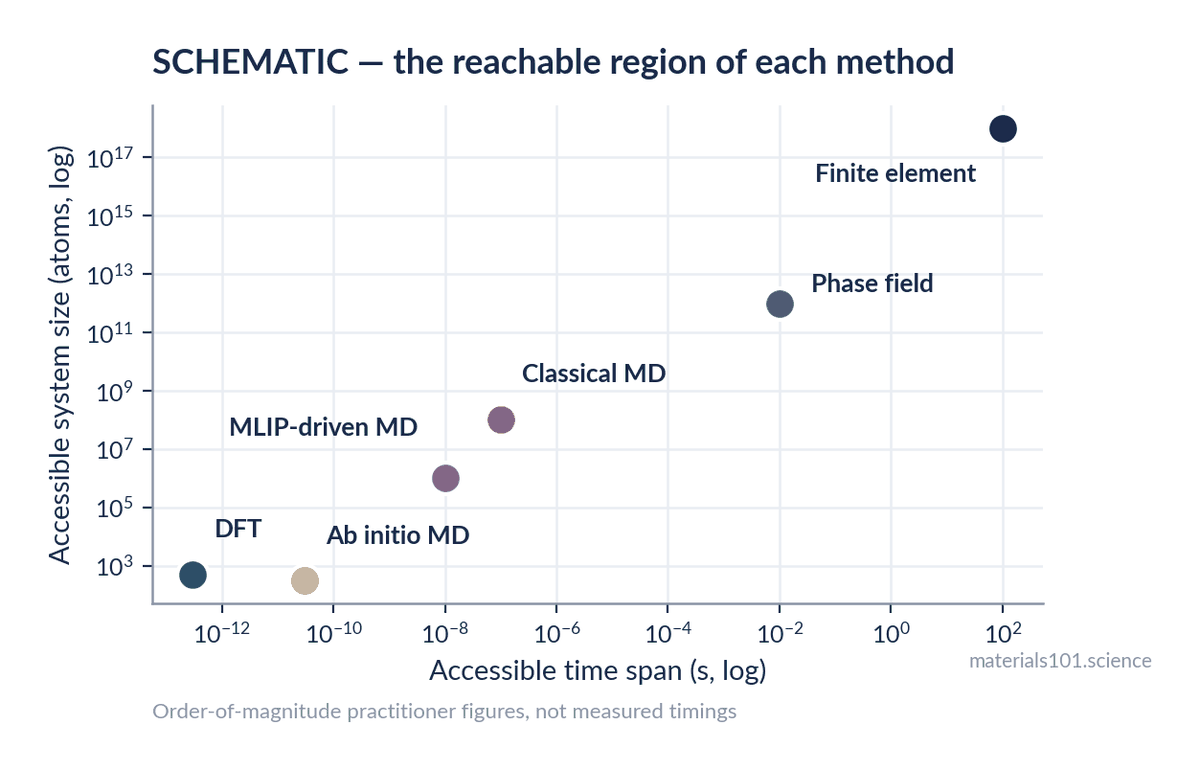
The numbers matter more than the categories. A DFT calculation of 200 atoms is a normal day’s work; 2,000 atoms is a project. An MD simulation of a million atoms for a nanosecond is routine on a modest cluster. That is four orders of magnitude in system size and at least three in time.
A decision procedure
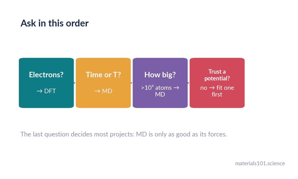
Ask these in order.
1. Does the answer involve electrons?
Band structure, optical absorption, magnetic moments, charge transfer, oxidation states, reaction barriers with bond breaking, core-level spectra. If yes, you need DFT. MD cannot give you these at all, because it has no electrons to give.
2. Does the answer involve temperature or time?
Diffusion coefficients, melting points, thermal conductivity, viscosity, phase transformation kinetics, mechanical response at a strain rate. If yes, you need MD — or DFT-derived parameters fed into something else.
3. How big does the system have to be?
A dislocation core needs a few thousand atoms to avoid its own image forces. A crack tip needs tens of thousands. A grain boundary network needs millions. Anything above a few thousand atoms rules out plain DFT.
4. Do you have a potential you trust?
This is the question that actually decides most projects. MD is only as good as its forces. If no reliable potential exists for your chemistry — a multicomponent alloy, an unusual oxide — then MD is not cheap, it is meaningless, and you either fit a potential first or restructure the question to fit DFT.
Going deeper
There is a fifth question, easy to miss: what timescale does the process actually take? MD integrates in femtosecond steps, so a microsecond trajectory is 10⁹ steps — feasible but expensive. A process with an activation barrier of 1 eV has a rate around 10⁻⁴ s⁻¹ at room temperature, so the expected waiting time is hours. You will never see it in MD, no matter how fast your potential. This is the rare event problem, and it is why accelerated methods exist: nudged elastic band for the barrier itself, transition state theory to convert it into a rate, metadynamics or hyperdynamics to bias the sampling, kinetic Monte Carlo to propagate a system through known events. Simply running longer is almost never the answer.
Ab initio MD: the expensive middle ground
You can do molecular dynamics with DFT forces, recomputing the electronic structure at every timestep. That is ab initio molecular dynamics, and it gives you finite-temperature dynamics with quantum-mechanical forces and no fitted potential.
The price is severe. A few hundred atoms for tens of picoseconds is a realistic AIMD campaign, which is a million times less trajectory than classical MD delivers for the same compute.
AIMD earns its cost when the electronic structure changes during the process: bond breaking and forming in a reaction, a liquid in which coordination is constantly changing, a metal-insulator transition, proton transfer. In those cases a fixed classical potential cannot describe what is happening even in principle.
This is precisely the niche machine-learned potentials have eaten. Train on AIMD snapshots, then run classical-speed MD with near-DFT forces — a few orders of magnitude more trajectory for the same cost. For many problems that formerly required AIMD, the honest answer in 2026 is: generate DFT data, fit a potential, run MD, and validate.
What each one cannot do
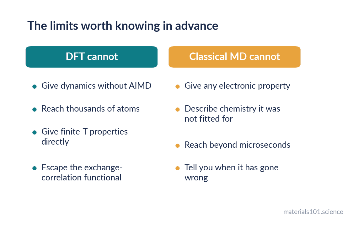
DFT cannot give you dynamics without AIMD; reach thousands of atoms; predict finite-temperature properties without extra machinery (phonons, quasi-harmonic approximation); or escape the exchange-correlation functional. Standard functionals underestimate band gaps for structural reasons and need explicit corrections for dispersion and strong correlation.
Classical MD cannot give you any electronic property; describe chemistry its potential was not fitted for; reach timescales beyond microseconds; or tell you when it has gone wrong — a classical potential extrapolates smoothly and confidently into nonsense.
Both inherit a reference. DFT inherits its functional; MD inherits its potential, which was probably fitted to DFT, which inherited its functional. It is worth remembering how far from experiment you are standing.
In practice
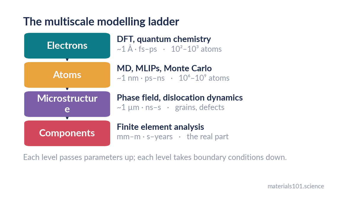
The common real workflow is a chain rather than a choice. DFT computes the energies of a few hundred configurations; a machine-learned potential is fitted to them; MD runs a million atoms for nanoseconds using that potential; and the resulting quantity — an elastic constant, a diffusion coefficient, an interface energy — becomes a parameter in a phase-field or finite-element model of the actual component. Each level takes its parameters from the level below and its boundary conditions from the level above. When someone asks which method to use, the useful reply is usually “which rung of that ladder is your question on?”
Common misconceptions
- “DFT is more accurate than MD.” They compute different things. DFT is more fundamental about electrons; a well-validated MD run is far more reliable about melting points than a 0 K DFT calculation.
- “MD is classical, so it is approximate, so it is worse.” MD with an accurate potential gives finite-temperature properties that DFT cannot reach at all. The approximation is in the forces, not the dynamics.
- “AIMD is the best of both.” It is the most expensive of both, and correct only when the electronic structure genuinely changes during the process.
- “Longer MD runs solve the timescale problem.” They do not. A 1 eV barrier means hours of real time; use accelerated sampling or transition state theory.
Key takeaways
- DFT solves for electrons in a fixed structure; MD propagates atoms in time using forces it is given.
- DFT handles 10²–10³ atoms and scales as roughly N³; MD handles 10⁵–10⁹ atoms and scales as roughly N.
- Ask in order: does it involve electrons, does it involve temperature or time, how big must the system be, and do you trust a potential for this chemistry.
- AIMD is justified when bonding changes during the process, and has largely been displaced by machine-learned potentials fitted to DFT.
- The rare event problem is not solved by longer runs; it needs barrier calculations or accelerated sampling.
Frequently asked questions
What is the difference between DFT and molecular dynamics?
DFT computes the electronic ground state of a fixed arrangement of atoms, giving energies, forces and electronic structure. Molecular dynamics integrates Newton’s equations to follow atoms over time at a temperature, using forces supplied by a potential. DFT gives you electrons; MD gives you dynamics.
Can molecular dynamics predict electronic properties?
No. Classical MD has no electrons in it. For band structures, optical properties or magnetic moments you need DFT, or ab initio MD if you also need finite-temperature dynamics.
When should I use ab initio molecular dynamics?
When the electronic structure changes during the process you are studying — bond breaking in a reaction, a liquid with fluctuating coordination, a metal-insulator transition. Otherwise a machine-learned potential fitted to DFT data gives orders of magnitude more trajectory for the same cost.
How many atoms can DFT handle?
Routinely a few hundred with plane-wave codes on a normal cluster; a thousand or more is a serious undertaking because cost scales as roughly the cube of the electron count. Classical MD reaches millions to billions.
Which method should I learn first?
Whichever matches the questions in your group, but learning DFT first makes the second easier: it teaches you where interatomic potentials come from and why their quality decides whether an MD result means anything.
Next read
- Density functional theory, explained without the math — how the electron side works
- Your first LAMMPS simulation, step by step — the dynamics side, hands on
- What is a machine-learned interatomic potential? — the bridge between the two
References
Both scale figures in this post are schematic and labelled as such; the system
sizes and cost ratios quoted in the table are order-of-magnitude practitioner
figures drawn from the references below rather than measured timings.
- R. M. Martin, Electronic Structure: Basic Theory and Practical Methods, 2nd ed., Cambridge University Press, 2020 — DFT scaling, practical system sizes, what electronic structure methods deliver.
- M. P. Allen and D. J. Tildesley, Computer Simulation of Liquids, 2nd ed., Oxford University Press, 2017 — molecular dynamics fundamentals, accessible timescales, ensemble properties.
- D. Marx and J. Hutter, Ab Initio Molecular Dynamics: Basic Theory and Advanced Methods, Cambridge University Press, 2009 — the scope and cost of AIMD.
- G. Henkelman, B. P. Uberuaga and H. Jónsson, A climbing image nudged elastic band method for finding saddle points and minimum energy paths, The Journal of Chemical Physics 113, 9901–9904 (2000). doi:10.1063/1.1329672 — the standard route around the rare event problem.
Written by Dinesh Varma, PhD scholar in computational materials science.
Spotted an error? Tell me — corrections are credited.