How Accurate Are Machine Learning Potentials, Really?

Ask how accurate machine-learned interatomic potentials are and you will usually be told a number like “a few meV per atom”. That number is true and almost useless, and the reason is visible in a single public leaderboard.

Take the top five models on Matbench Discovery. Their energy errors differ by 11% — statistically, they are the same model. Their errors on thermal conductivity differ by 83%. Same five models, two metrics, and essentially no relationship between them.

By the end of this post you will know what published accuracy numbers do and do not tell you, and what to measure on your own system before trusting a potential with a result.

In this post:

• The numbers, from a public leaderboard
• Why energy error and physical fidelity come apart
• What “a few meV per atom” actually means
• The error that matters is in the tail
• A validation protocol you can run in a day

The numbers

Matbench Discovery evaluates universal interatomic potentials on their ability to predict thermodynamic stability, using DFT as the reference [1]. Here are the top five by its composite score, as the leaderboard stood on 12 September 2026 [2].

Model	F1 (stability)	DAF	Energy MAE (eV/atom)	κSRME
PET-OAM-XL	0.924	6.075	0.019	0.119
eSEN-30M-OAM	0.925	6.069	0.018	0.170
EquFlash	0.919	5.983	0.019	0.158
Nequip-OAM-XL	0.906	5.869	0.020	0.125
MatRIS-10M-OAM	0.921	6.039	0.019	0.218

Three of those columns need a sentence each.

F1 measures how well the model classifies a structure as thermodynamically stable or not, against DFT. All five sit between 0.906 and 0.925 — a spread of 2%.

DAF, the discovery acceleration factor, is how much more often the model’s picks are stable than random selection from the same pool. Around 6× for all five.

κ_SRME is the symmetric relative mean error in lattice thermal conductivity, derived from the phonons the model predicts. Lower is better. Here the five spread from 0.119 to 0.218.

Why the two metrics come apart

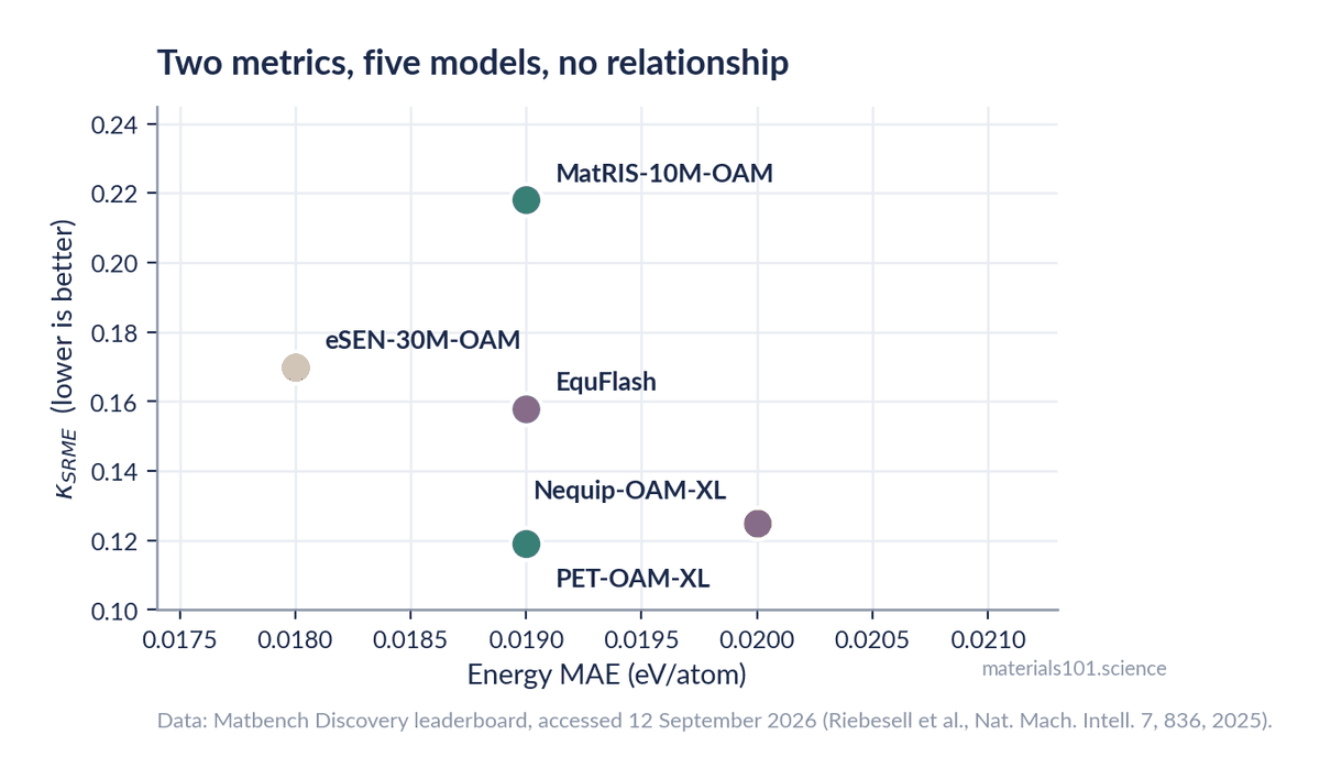
Look at the two extremes. PET-OAM-XL and MatRIS-10M-OAM both post an energy MAE of 0.019 eV/atom — identical to the precision quoted. On thermal conductivity, one is nearly twice as wrong as the other.

The reason is what each metric probes. Energy MAE asks whether the model gets the value of the energy right at a set of configurations. Thermal conductivity asks whether it gets the second derivative of that energy surface right — the force constants that set phonon frequencies and lifetimes. A surface can sit at almost exactly the right height everywhere and still have the wrong curvature.

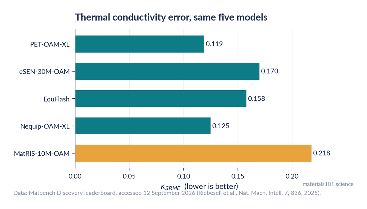
This is not a flaw in the benchmark — it is the benchmark doing its job. It is a flaw in the habit of quoting one number for “accuracy”.

What “a few meV per atom” actually means

Put 0.019 eV/atom in context.

Against chemical accuracy. 1 kcal/mol is about 43 meV. So 19 meV/atom is inside chemical accuracy per atom — but errors do not necessarily stay per-atom when you compare structures with different atom counts, and formation-energy differences between competing polymorphs are often 10–50 meV/atom. At that scale a 19 meV error can invert the predicted stability ordering of two phases.

Against thermal energy. k_BT at room temperature is about 25 meV. The model’s typical error is comparable to the thermal energy driving the physics you are simulating.

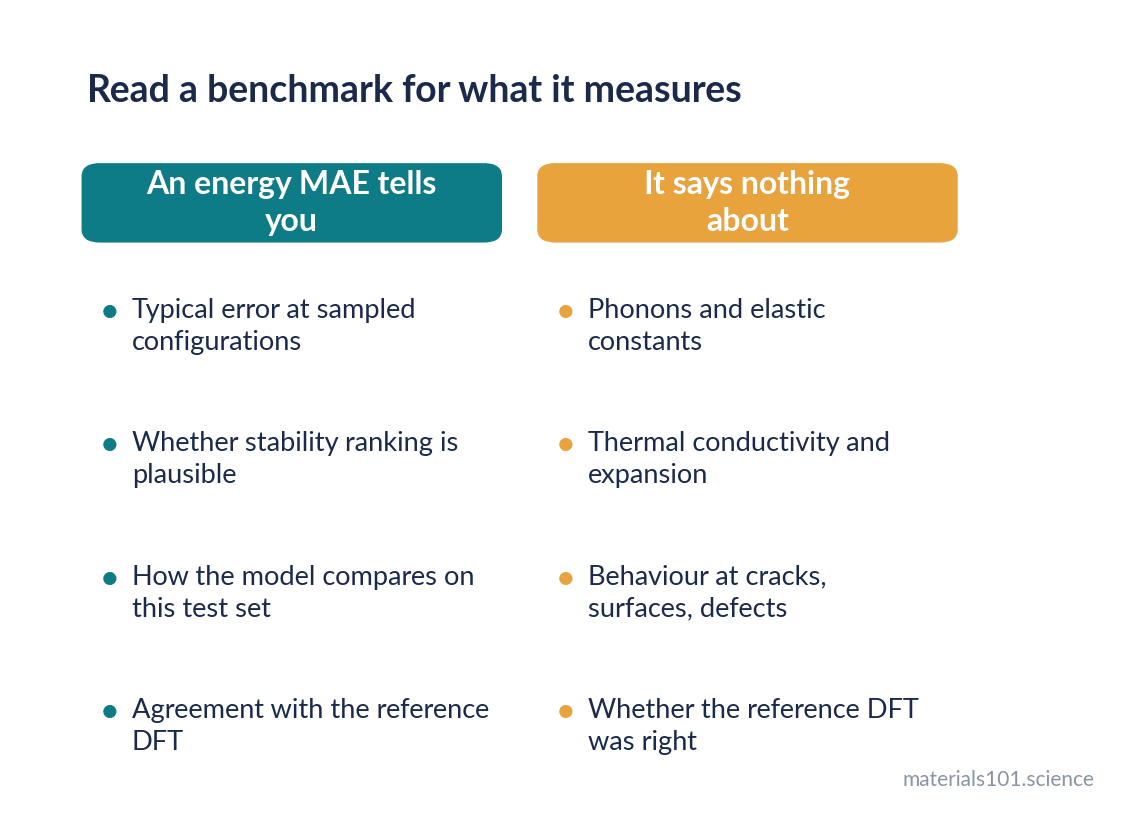
Against the reference. Most importantly, these errors are measured against DFT, not reality. A model that reproduced PBE perfectly would inherit PBE’s own errors: lattice parameters about 1% large, systematically underestimated band gaps, poor dispersion without a correction. Zero benchmark error would still leave you with DFT’s accuracy, not nature’s.

So “a few meV per atom” means: good enough to rank most structures, marginal for closely competing polymorphs, and silent about whether the phonons, elastic constants or transport properties are right.

The error that matters is in the tail

Mean absolute error is a mean. Simulations do not fail on average configurations; they fail on the rare ones.

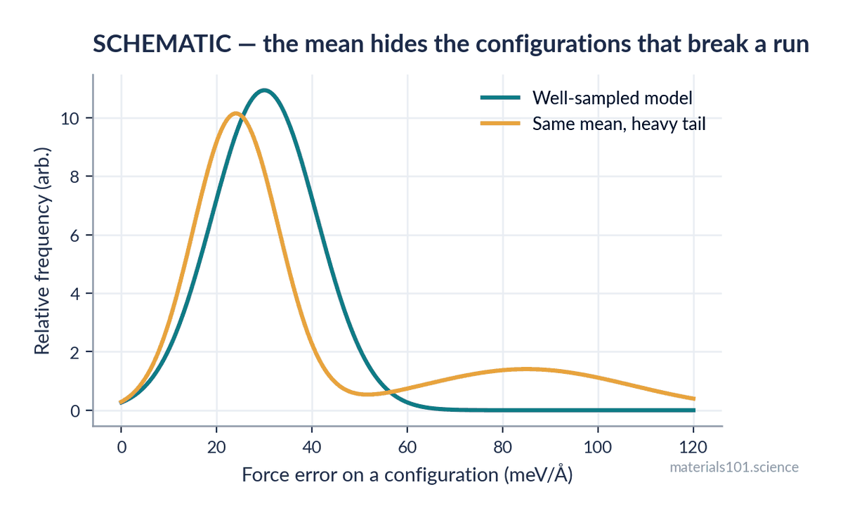
Consider a crack-tip simulation. The vast majority of local environments are near-equilibrium bulk, where the model is excellent. A tiny fraction are severely strained bonds at the tip — precisely the configurations a well-equilibrated training set rarely samples. The MAE over the whole trajectory stays beautiful. The crack propagates at the wrong stress.

The same argument applies to melting, defect formation, transition states and surfaces. In every case the physics you are studying lives in the tail of the configuration distribution, which is the part of the training distribution that is thinnest.

Two practical consequences. First, report error distributions rather than means alone — a 99th percentile force error tells a reader far more than an MAE. Second, ensembles are the cheapest uncertainty estimate available: train three to five models with different seeds, and take their disagreement on a configuration as a proxy for error. It correlates well enough with true error to flag when your simulation has wandered out of distribution, and it costs nothing but training time.

A validation protocol you can run in a day

Before a potential is allowed to produce a number you will publish:

1. Reproduce the reference. Compute lattice parameter, cohesive energy and bulk modulus with the potential and with the DFT it was trained on. Agreement here is table stakes; disagreement means something is wrong with your setup, not the model.
2. Compute the phonon spectrum. Imaginary modes in a structure known to be stable mean the curvature is wrong, and no amount of good force MAE rescues that. This one test would catch most of the κ_SRME spread above.
3. Check elastic constants against experiment where they exist. Second derivatives again, and independent of the DFT reference.
4. Run an ensemble on your actual trajectory and plot uncertainty against time. A rising trend means the simulation is leaving the training distribution.
5. Validate one property you did not fit. Melting point, defect formation energy, surface energy — anything measured. This is the only test that speaks to reality rather than to DFT.
6. State all of it in the paper. “We used MACE-MP” is not a method; which version, which fine-tuning data, and which of these checks passed is.

Common misconceptions

• “State of the art on the leaderboard means best for my system.” Leaderboards average over a broad structure set. Your system is one point in it, and model rankings reorder on narrow chemistries.
• “Low force MAE means good dynamics.” Force error is a first derivative; dynamics and transport depend on higher ones. The κ_SRME spread above is that gap, quantified.
• “Benchmark accuracy is physical accuracy.” All of these numbers are measured against DFT. The model inherits every error of its reference.
• “Uncertainty estimation is for careful people.” It is how you find out that your simulation left the training distribution 200 picoseconds ago.

Key takeaways

• Across the top five models on Matbench Discovery, energy MAE varies by 11% while thermal conductivity error varies by 83% — accuracy is property-specific.
• Energy and force errors constrain the zeroth and first derivatives of the energy surface; phonons, elastic constants and transport depend on higher ones, which nothing in the loss function controls.
• 0.019 eV/atom is comparable to k_BT at room temperature and to the energy differences between competing polymorphs.
• All published errors are relative to DFT, so a perfect score still carries DFT’s own errors.
• What breaks a simulation is the tail of the error distribution, not its mean; ensembles are the cheapest way to see it coming.

Frequently asked questions

How accurate are machine learning interatomic potentials?
On broad benchmarks, the leading universal models reach around 0.018–0.020 eV/atom on the energy metric and classify thermodynamic stability with an F1 near 0.92 against DFT. But their errors on phonon-derived thermal conductivity differ by nearly a factor of two, so accuracy depends entirely on which property you need.

Are machine learning potentials as accurate as DFT?
Inside their training distribution they approach the DFT they were trained on for energies and forces. They are not more accurate than that DFT, and they say nothing about electronic properties. Outside the training distribution they extrapolate without warning.

What is κ_SRME in Matbench Discovery?
The symmetric relative mean error in lattice thermal conductivity, computed from the phonons the model predicts. It probes the second and higher derivatives of the energy surface, which is why it separates models that look identical on energy error.

How do I know if a potential is reliable for my system?
Reproduce lattice parameter, cohesive energy and bulk modulus against your DFT; compute the phonon spectrum and check for spurious imaginary modes; compare elastic constants to experiment; run an ensemble and watch the disagreement along your trajectory; and validate one property you did not fit.

Should I use a foundation model or fit my own potential?
Start with a foundation model for orientation and screening. For quantitative results on one system, fine-tune it on a few hundred of your own DFT configurations, then re-run the validation checks.

Next read

• What is a machine-learned interatomic potential? — how these models work, if you want the mechanism first
• Density functional theory, explained without the math — the reference all of these errors are measured against

References

Figures 1 and 2 plot leaderboard values retrieved on 12 September 2026; figure 4
is a labelled schematic illustrating a distributional argument, with no data.
Leaderboard rankings change — check the live page before quoting these numbers.

1. J. Riebesell, R. E. A. Goodall, P. Benner et al., A framework to evaluate machine learning crystal stability predictions, Nature Machine Intelligence 7, 836–847 (2025). doi:10.1038/s42256-025-01055-1
2. Matbench Discovery leaderboard, matbench-discovery.materialsproject.org, accessed 12 September 2026 — source of the F1, DAF, energy MAE and κ_SRME values in the table and figures.
3. S. Batzner et al., E(3)-equivariant graph neural networks for data-efficient and accurate interatomic potentials, Nature Communications 13, 2453 (2022). doi:10.1038/s41467-022-29939-5
4. I. Batatia, D. P. Kovács, G. N. C. Simm, C. Ortner and G. Csányi, MACE: Higher Order Equivariant Message Passing Neural Networks for Fast and Accurate Force Fields, NeurIPS (2022).

---

Written by Dinesh Varma, PhD scholar in computational materials science, whose PhD work benchmarks machine-learned interatomic potentials.
Spotted an error? Tell me — corrections are credited.