

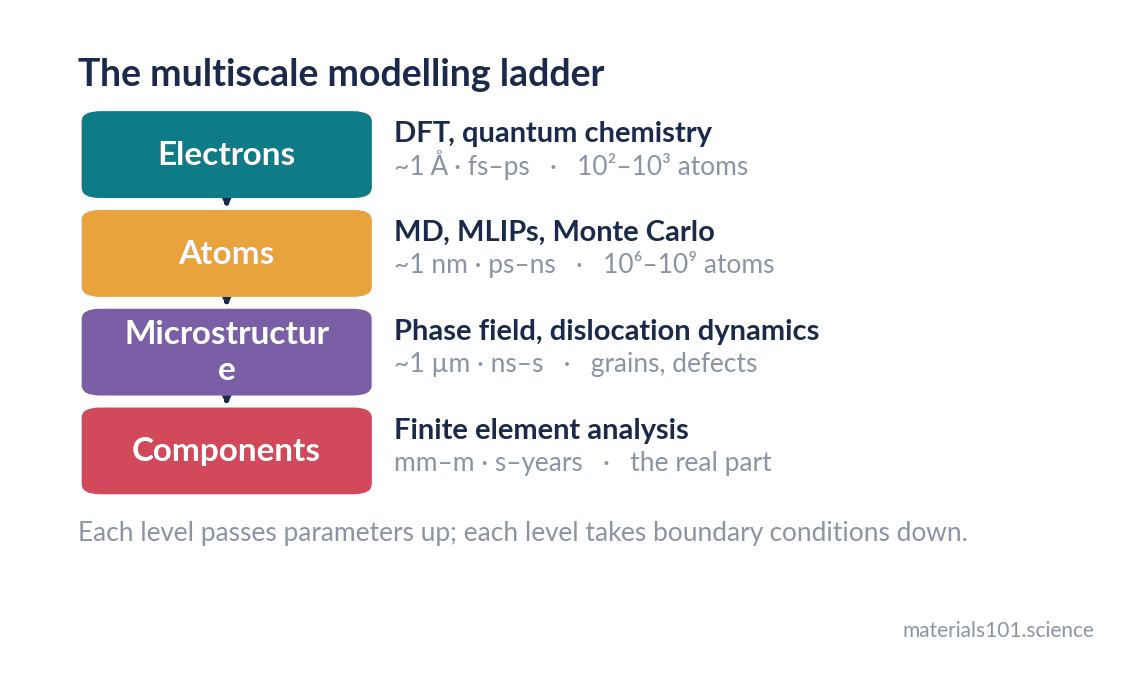
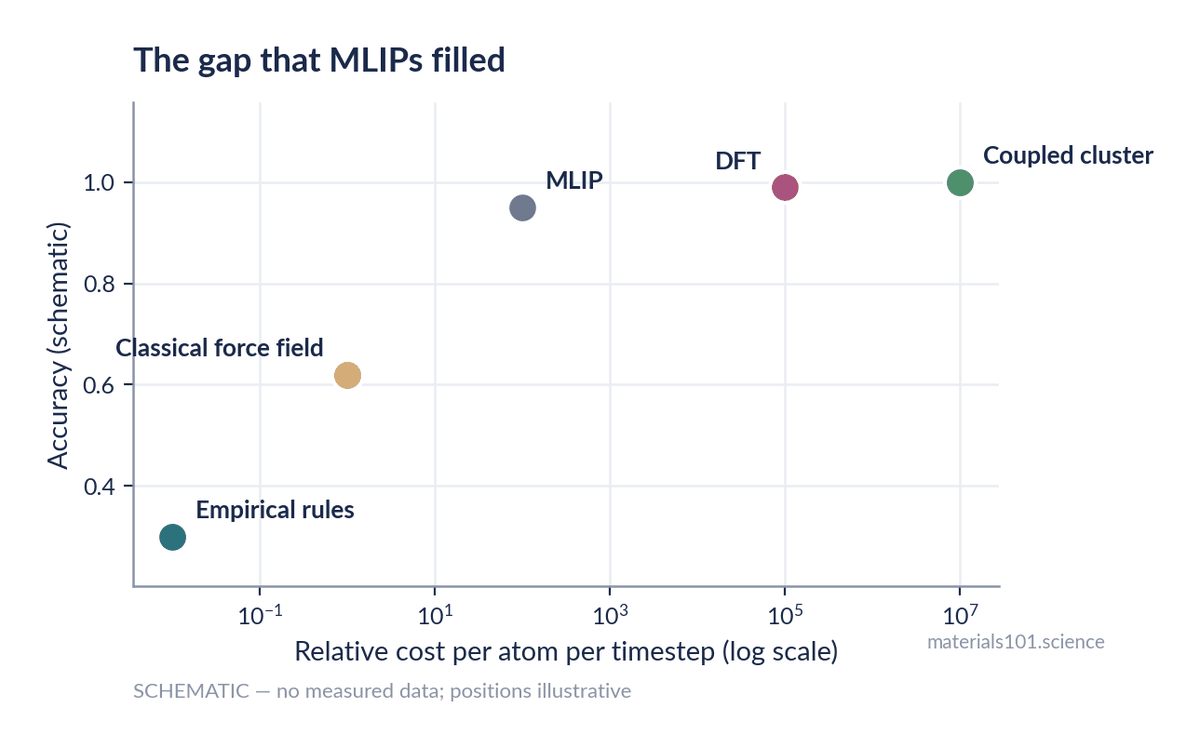
Here is the trade every atomistic simulation used to force on you. Density functional theory gives you forces you can believe, on a few hundred atoms, for a few picoseconds. A classical force field gives you millions of atoms for nanoseconds, using a functional form someone chose in 1985 and fitted to six numbers.
For thirty years there was nothing in between. Machine-learned interatomic potentials are what filled that gap, and they changed which questions are askable.
By the end of this post you will be able to explain what a machine-learned interatomic potential is, where its enormous speed advantage actually comes from, and — the part that matters most in practice — the specific way it fails.
In this post:
- The one-sentence definition, and what it hides
- How an MLIP sees an atom
- Where the speed comes from
- The families you will meet: GAP, ACE, NequIP, MACE, and the foundation models
- How MLIPs fail, and how to catch it
What is a machine-learned interatomic potential?
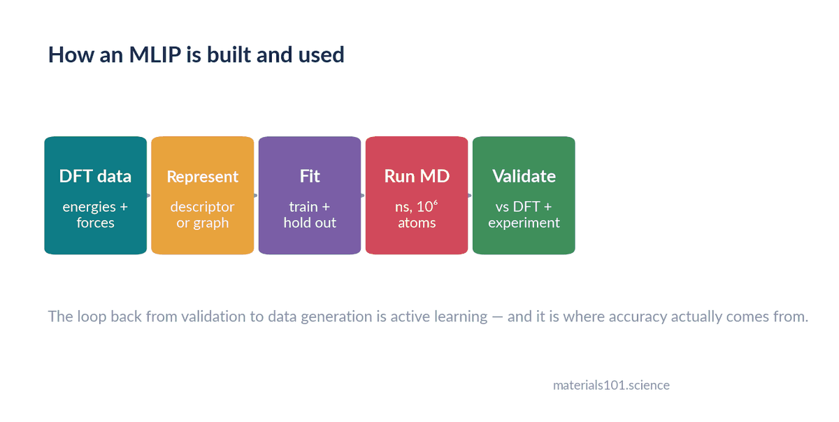
A machine-learned interatomic potential is a regression model that predicts the energy and forces of an atomic configuration, trained on energies and forces computed with quantum mechanics — almost always DFT. You give it the positions and species of the atoms; it gives you back the total energy and the force on every atom, fast enough to run molecular dynamics.
That is the whole idea. Everything interesting is in two design choices: how the model describes an atom’s surroundings, and how it maps that description to energy.
The critical assumption underneath both is locality. The total energy is written as a sum of atomic contributions, and each atom’s contribution depends only on the neighbours inside a cutoff radius, typically 4–6 Å:
Etotal = Σi Ei(local environment of atom i)
This is an approximation, and it is the reason the whole approach is fast — but it is also why long-range electrostatics, charge transfer between distant regions, and metallic screening effects need explicit extra treatment. A plain local MLIP does not know about them.
How an MLIP sees an atom
A neural network cannot take raw Cartesian coordinates. Rotate the whole system and the energy must not change; swap two identical atoms and the energy must not change; translate everything a metre to the left and nothing changes. Those invariances have to be built in, not learned, or the model will waste its capacity learning geometry instead of chemistry.
The traditional answer is a descriptor: a fixed mathematical fingerprint of the local environment that is invariant by construction. Behler–Parrinello symmetry functions (ACSF) [1] and the smooth overlap of atomic positions (SOAP) [2] are the two you will meet most. Both encode “what is around this atom, at what distances and angles” in a vector of a few hundred numbers.
The modern answer is a message-passing graph neural network. Atoms are nodes, neighbours within the cutoff are edges, and the model learns its own representation by passing information along those edges. Equivariant architectures go further: instead of throwing away directional information to achieve invariance, they carry vectors and higher-order tensors through the network in a way that rotates correctly with the system. That turns out to be dramatically more data-efficient — equivariant models reach a given accuracy with roughly an order of magnitude fewer training structures than their invariant predecessors.
Where the speed comes from
An MLIP is typically three to five orders of magnitude faster than the DFT it was trained on. It is worth understanding why, because the reason also explains the limitations.
DFT solves for the electronic structure at every single step. Even with clever algorithms, the cost scales as roughly N³ with the number of electrons, and every timestep starts a fresh self-consistent field cycle. There is no memory: yesterday’s converged density does not help with today’s new configuration except as a starting guess.
An MLIP does the quantum mechanics once, offline, on a training set. At run time there are no electrons at all — just a fitted function of neighbour positions, evaluated per atom, scaling linearly with system size and parallelising almost perfectly. You have moved the expensive part from the simulation into the training.
Going deeper
The accuracy figures usually quoted — of order 1–5 meV/atom for energies and tens of meV/Å for forces against the reference DFT — are typical of what the original papers report on their own held-out test sets [3–6], not a universal specification. Always read them as “this model, this training set, this system”. Two cautions. First, those errors are measured against DFT, not reality — an MLIP that reproduces PBE perfectly inherits every one of PBE’s own errors, including its systematic underbinding and its lattice constants that run about 1% large. Second, a low mean error hides everything: what breaks a simulation is the rare configuration with a large error, not the average one. Look at the error distribution’s tail, and look at it for the configurations your simulation will actually visit.
The families you will meet
GAP (Gaussian Approximation Potentials) [3] use SOAP descriptors with Gaussian process regression. Excellent accuracy and built-in uncertainty estimates; the cost grows with the number of training points, which limits how large the training set can practically get.
ACE (Atomic Cluster Expansion) [4] uses a systematic polynomial expansion of the local environment. It is fast at evaluation, has a clean mathematical basis, and gives you a knob — the body order and polynomial degree — to trade accuracy for speed deliberately rather than by trial and error.
NequIP and Allegro [5] are equivariant graph networks, and they made the data-efficiency argument convincingly: high accuracy from a few hundred to a few thousand DFT structures rather than tens of thousands.
MACE [6] combines the equivariant message-passing idea with a higher-body-order expansion, which lets it reach comparable accuracy with fewer message-passing layers — and fewer layers means a smaller effective receptive field and better parallel scaling.
Foundation models — MACE-MP, CHGNet [7], M3GNet [8] and their relatives — are trained on very large public DFT databases covering most of the periodic table. You can run one on a system it has never seen without training anything. They are extraordinarily useful as a starting point or a first look, and they are usually not as accurate on your specific system as a potential fitted to your own data. The realistic workflow is to start from a foundation model and fine-tune it on a few hundred of your own configurations.
How MLIPs fail
This is the section that matters, and it is the one most tutorials skip.
A classical force field fails loudly. Push it into a regime it was not designed for and the energy blows up, atoms fly apart, and you notice within a few hundred steps.
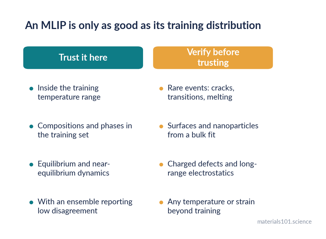
An MLIP fails quietly. Presented with a configuration unlike anything in its training set, it does not know it is extrapolating. It returns a perfectly plausible-looking energy and a perfectly plausible-looking force — and both are wrong. Your simulation runs to completion, produces smooth trajectories and a tidy plot, and the plot is fiction.
The situations where this bites are predictable:
- Temperatures above the training range. Train at 300 K, run at 1200 K, and the model is inventing.
- Rare events. Crack tips, transition states, defect formation and melting all involve configurations that a well-equilibrated training run rarely samples — which is exactly why they are missing from the training set.
- Compositions and phases outside the set. A potential fitted to bulk FCC copper knows nothing useful about a surface, a nanoparticle, or an oxide.
- Long-range interactions. Charged defects, polar surfaces and ionic systems need explicit electrostatics; the local cutoff cannot supply them.
The defences are equally predictable, and worth building in from the start. Use an ensemble of models trained with different seeds and treat their disagreement on a configuration as an uncertainty estimate — cheap, and it works. Use active learning: run the simulation, flag the high-uncertainty configurations, compute those with DFT, add them to the training set, retrain, repeat. And always validate on physical properties you did not fit — elastic constants, phonon spectra, melting point, defect formation energies — rather than only on held-out energies and forces.
In practice
A reasonable default workflow in 2026: start from a foundation model such as MACE-MP; run a short simulation of your actual system; use ensemble disagreement or a committee to select 200–500 configurations for DFT; fine-tune on those; then validate against at least one measured property before you trust a single production result. That whole loop costs a fraction of the DFT you would otherwise have run, and it is the difference between a potential that works and one that merely runs.
Common misconceptions
- “An MLIP is as accurate as DFT.” It is as accurate as the DFT it was trained on, inside its training distribution. Both of those qualifiers do real work.
- “More training data always helps.” Diversity helps; redundancy does not. Ten thousand configurations from one equilibrium trajectory teach a model less than five hundred well-chosen ones spanning temperatures, strains and defects.
- “Foundation models made fitting your own potential obsolete.” They made the starting point much better. For quantitative work on a specific system, fine-tuning on your own data still wins.
Key takeaways
- An MLIP is a regression model that predicts energies and forces from atomic positions, trained on DFT data, and assumes energy is a sum of local atomic contributions.
- The speed advantage — three to five orders of magnitude — comes from doing the quantum mechanics once, offline, instead of at every timestep.
- Equivariant graph networks such as NequIP and MACE reach a given accuracy with far less training data than descriptor-based models.
- MLIPs fail silently outside their training distribution, so uncertainty estimates, active learning and physical validation are not optional extras.
- Foundation models are an excellent starting point and a poor final answer for a specific system.
Frequently asked questions
What is a machine-learned interatomic potential in simple terms?
It is a model that learns the relationship between where atoms are and what the energy and forces are, using quantum-mechanical calculations as training data. Once trained, it predicts forces fast enough for molecular dynamics on millions of atoms, without solving the electronic structure again.
How much faster is an MLIP than DFT?
Typically three to five orders of magnitude per atom per timestep, and it scales linearly with system size rather than cubically. That converts a calculation of hundreds of atoms for picoseconds into millions of atoms for nanoseconds.
Are machine learning potentials accurate?
Inside their training distribution, yes — commonly a few meV/atom in energy and tens of meV/Å in force against the reference DFT. Outside it, they extrapolate without warning, which is why uncertainty estimation matters more than headline accuracy numbers.
Which MLIP should I use?
For a first look at almost anything, start with a foundation model such as MACE-MP or CHGNet. For production work on one system, fine-tune it or fit a dedicated MACE or ACE potential on your own DFT data, then validate against a property you did not fit.
Do I still need DFT if I have an MLIP?
Yes. DFT generates the training data, provides the reference for validation, and handles electronic properties — band structures, charge densities, magnetic states — that a potential does not predict at all.
References
The cost and accuracy positions in the trade-off figure are schematic and the
figure says so; the orders of magnitude are the ranges reported across the papers
below rather than a single benchmark. Where this post quotes an accuracy figure it
is the range those papers report on their own test sets.
- J. Behler and M. Parrinello, Generalized Neural-Network Representation of High-Dimensional Potential-Energy Surfaces, Phys. Rev. Lett. 98, 146401 (2007). doi:10.1103/PhysRevLett.98.146401
- A. P. Bartók, R. Kondor and G. Csányi, On representing chemical environments, Phys. Rev. B 87, 184115 (2013). doi:10.1103/PhysRevB.87.184115
- A. P. Bartók, M. C. Payne, R. Kondor and G. Csányi, Gaussian Approximation Potentials: The Accuracy of Quantum Mechanics, without the Electrons, Phys. Rev. Lett. 104, 136403 (2010). doi:10.1103/PhysRevLett.104.136403
- R. Drautz, Atomic cluster expansion for accurate and transferable interatomic potentials, Phys. Rev. B 99, 014104 (2019). doi:10.1103/PhysRevB.99.014104
- S. Batzner et al., E(3)-equivariant graph neural networks for data-efficient and accurate interatomic potentials, Nat. Commun. 13, 2453 (2022). doi:10.1038/s41467-022-29939-5
- I. Batatia, D. P. Kovács, G. N. C. Simm, C. Ortner and G. Csányi, MACE: Higher Order Equivariant Message Passing Neural Networks for Fast and Accurate Force Fields, NeurIPS (2022).
- B. Deng et al., CHGNet as a pretrained universal neural network potential for charge-informed atomistic modelling, Nat. Mach. Intell. 5 (2023). doi:10.1038/s42256-023-00716-3
- C. Chen and S. P. Ong, A universal graph deep learning interatomic potential for the periodic table, Nat. Comput. Sci. 2 (2022). doi:10.1038/s43588-022-00349-3
Next read
- Density functional theory, explained without the math — where the training data comes from
- How accurate are machine learning potentials, really? — the benchmark numbers, with the caveats
- Your first LAMMPS simulation, step by step — the hands-on version of this post
Written by Dinesh Varma, PhD scholar in computational materials science, whose PhD work benchmarks machine-learned interatomic potentials.
Spotted an error? Tell me — corrections are credited.